Assignment 02
ParaView
Due: Feb. 13, 2017 11:59:59 PM
Graded: Feb. 20, 2017
Percentage of Grade: 7%
Assignment Description: Finalized
- Prerequisites
- Getting Started
- Part 1: Loading Simple Data
- Part 2: Loading a 2d Image
- Part 3: Working with Polygonal Meshes
- Part 4: Visualizing Unstructured Meshes
- Part 5: Visualizing 3D Images
- Grading
Instructor’s note: this assignment is adapted from an exercise by Julian Tierny. While this assignment has changed significantly, you may find referring to it helpful for extra tips on ParaView.
Prerequisites
This assignment requires you to install a recent version of ParaView. Version 5.1 or higher should be sufficient. Binary installers exist on most platforms, but you do need administrator privileges to install it.
Please contact me if you need this installed on a department lab machine and we can arrange a solution.
In addition you will need the following datasets: data02.zip
Getting Started
ParaView is an open source multiple-platform application for interactive scientific visualization. It can be seen as a user-interface front-end to the VTK library. Notable features of ParaView are its support for highly parallelized and distributed processing as well as its remote visualization capabilities.
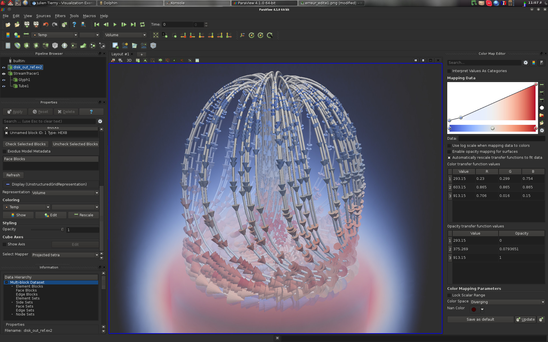
As shown in the above screenshot, the user interface is divided into several panels (yours may vary a bit depending on your configuration):
-
Pipeline Browser (top left): This panel lists the different data-sets that have been loaded by the user as well as the filter effects that have been applied to them;
-
Properties (middle left): This panel enables to interact with the visualization properties of the selected item in the pipeline browser;
-
Information (bottom left): This panel displays statistics and properties about the selected item in the pipeline browser;
-
Color Map Editor (right): This panel enables to interact with color maps; and
-
Central View (middle): This is where the actual visualization happens! Note that several tabs can be opened, to alternate between several visualizations using the split horizontal/split vertical buttons in the top right of this view.
Along the interactions, other panels can optionally be displayed, for instance to visualize and interact with planar layouts such as charts or histograms.
ParaView follows VTK’s visualization pipeline philosophy. In this paradigm, a visualization is obtained by applying a sequence of processing tasks on one or several datasets. In VTK, processing tasks are encapsulated by filters. Each filter takes some data on its input and delivers some data on its output. In the above example:
-
1 data-set has been loaded (disk_out_ref.ex2);
-
1 filter (called Stream Tracer) has been applied on the input, yielding a pipeline object named StreamTracer1;
-
2 filters have been applied on the pipeline object StreamTracer1, yielding two new pipeline objects: Glyph1 and Tube1.
Pipeline objects can be visualized or hidden by clicking on the eye icon on the left of each object.
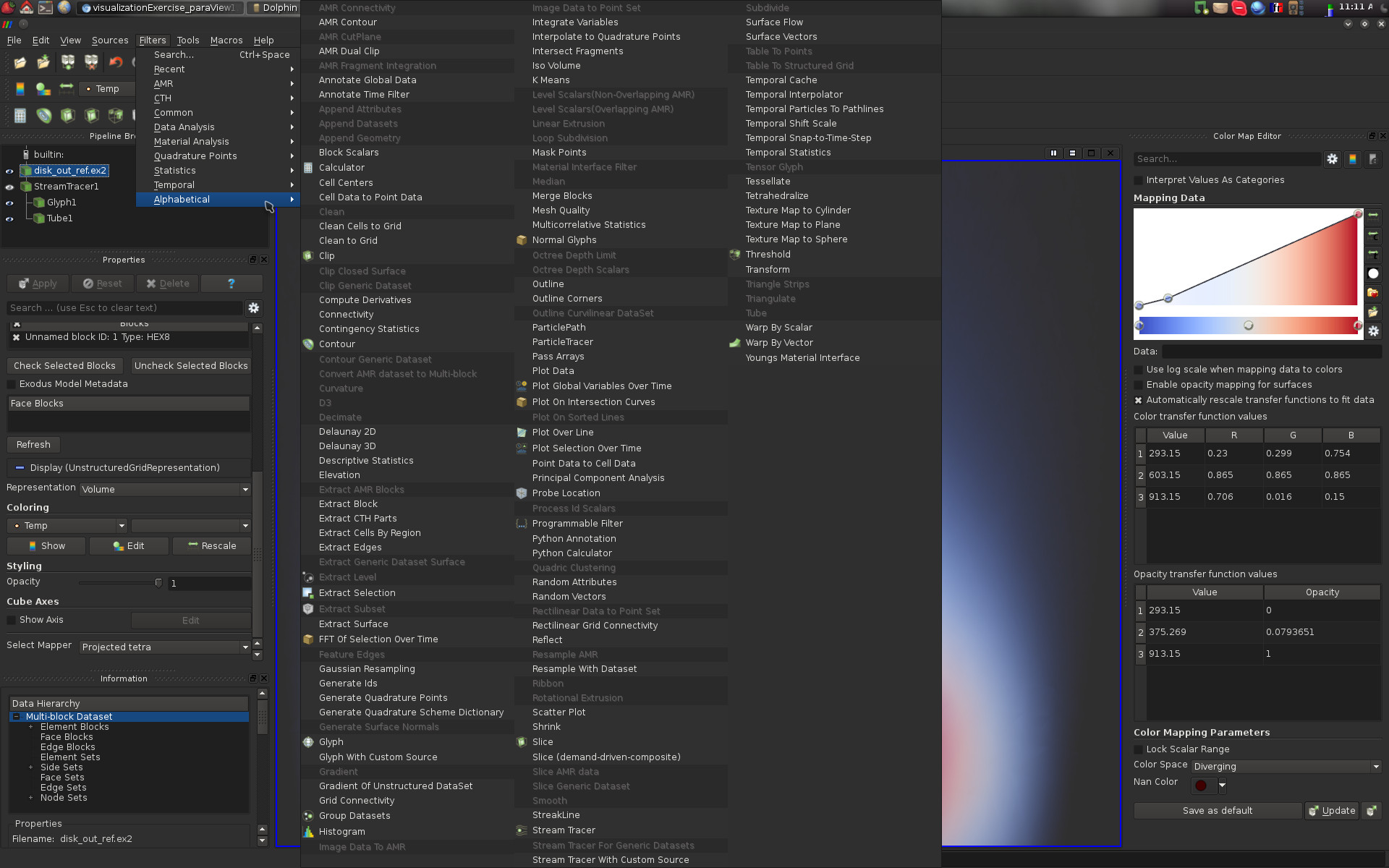
Given a pipeline object, a large selection of filters can be applied to it. In the following screen-shot, the list of default filters is displayed. Only those that can be applied to the selected pipeline object are not shaded and can consequently be executed. Note that with the menu Filters->Search… you can easily search for filters by typing a few letters contained in their name.
To load a data-set in ParaView, use the following menu File->Open. To
save your current pipeline, use the following menu File->Save State.
At certain places in this assignment, I will request that you save and
git commit state files demonstrating you accomplished the tasks of the
assignment. I will also request that include a file A02report.txt
that answers certain questions.
Now, let’s get the exercise started.
Part 1: Loading Simple Data
ParaView can visualize many types of datasets, from both very simple to very complicated. First, File->Open the dataset from Assignment 01 (data01.txt) in ParaView. In the Properties panel, make sure that you uncheck Have Headers before you hit Apply, since this text file is just a flat list of numbers.
You’ll quickly see…a SpreadSheetView! Given that ParaView does not know much about the data you’re trying to visualize, the best it can do is show you the raw data. If you’ve loaded this data correctly, you should that the maximum row ID is 229 (as there are 230 rows, counting from 0).
To get some basic visualization up, split the center window vertically. A dialogue should appear that looks like:

Click on “Histogram View”. With this view highlighted (you should see a blue border around it), click on the (greyed-out) eye next to `data01.txt in the Pipeline Browser to enable this dataset to be drawn in the histogram. One problem is that the histogram, by default, has too many bins. In our case, we have exactly 100 possibilities (numbers between 0 and 99), so in the Properties panel, set the bin count to 100. This should give you a histogram that looks like the one you generated in Assignment 01.
The difference is that this histogram has axes and is interactive (you
can zoom and pan with the mouse). The bins are not exactly labeled
right, but you use them to roughyly estimate the frequency of values by
hovering over with your mouse. In A02report.txt answer:
-
Which number occurred the most frequently and how many times did it occur?
-
How many numbers were never used by the class?
Part 2: Loading a 2d Image
Next, we’ll be working with the data file 2d.vti. Files that end in
.vt* are VTK file formats, the last letter of which indicates what
type of file. .vti files are Images.
Open up ParaView and load 2d.vti. This is a grayscale image that
samples a 2D scalar field. By default, ParaView automatically maps the
scalar values to color. You should be seeing something like:
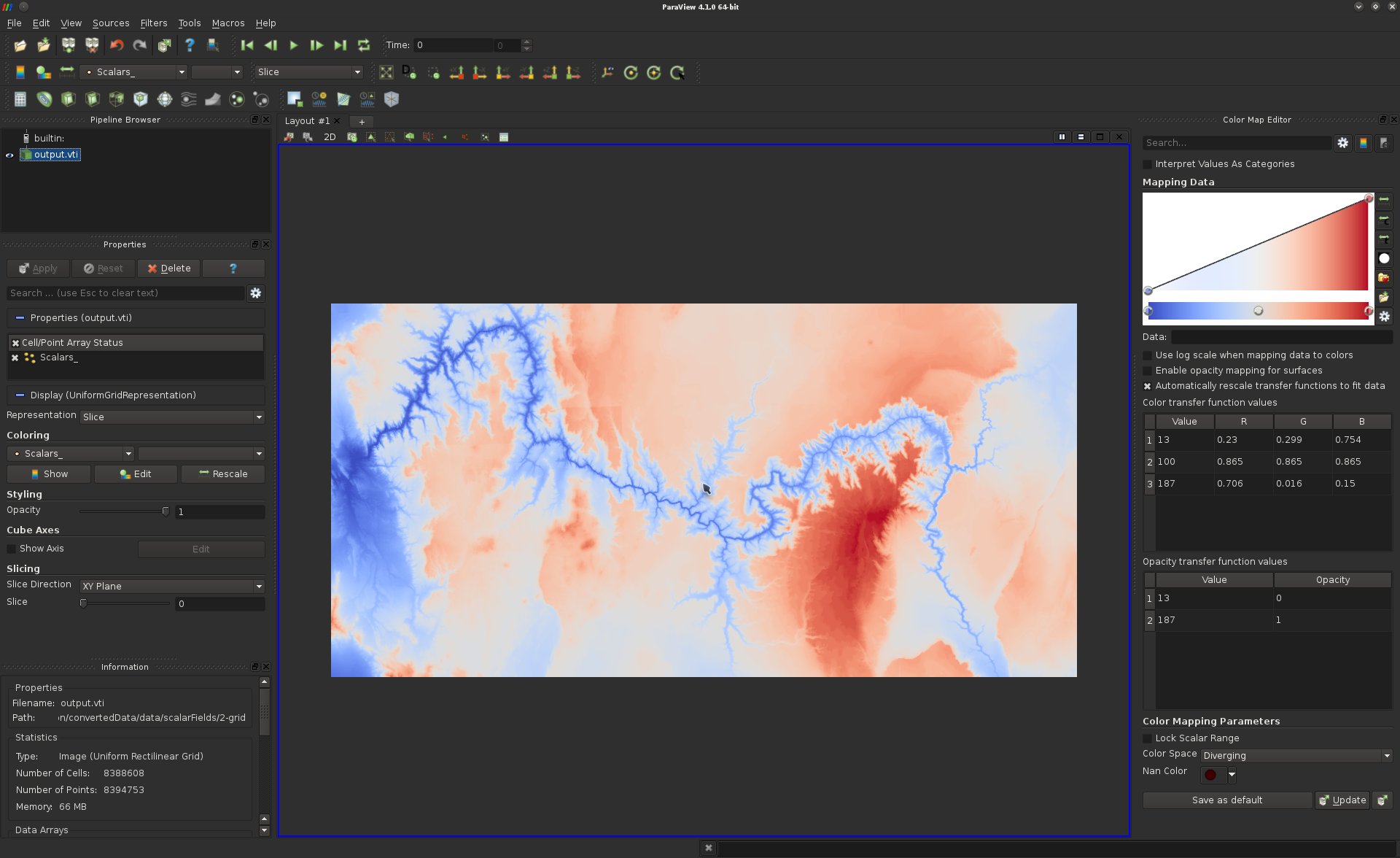
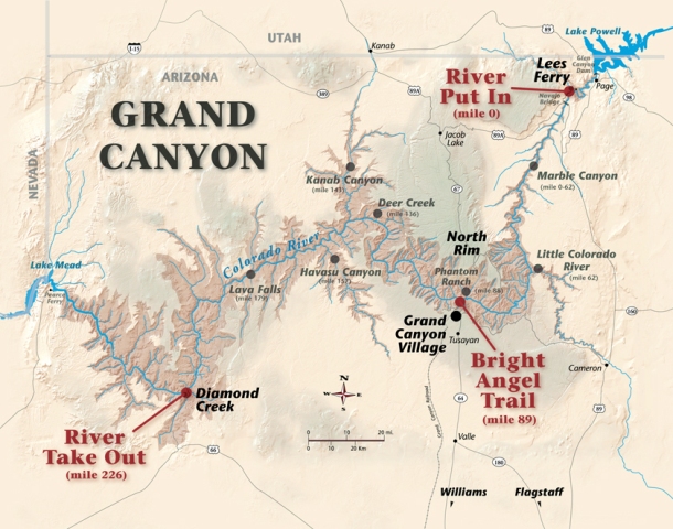
This image has pixels that correspond to height values associated with the Grand Canyon (see a map here to compare). Note that if you click and drag with the mouse you can reposition it. Since this data is two-dimensional, ParaView by default loads the render view in 2D mode (you’ll see this in the upper left of the view).
Let’s try working with a simple Filter. Go to Filters->Common->Threshold and add a Threshold filter. This subselects only those points that have values with a particular range. You’ll see the minimum and maximum initialize to the range of data.
What we’d like to do is try to only select the pixels that correspond to
the canyon itself. To aid in deciding which values are above the canyon
flow, it might be helpful to use a histogram. Split the view
vertically, and in the view below again create a histogram. Select this
view and click on the eye next to 2d.vti. Adjust the number of bins
based on the minimum and maximum of the data so that you have exactly
the right number of bins (you’ll know you’re correct where there are no
gaps between bars in the histogram). Based on the histogram, select the
top render view, disable the view of the entire dataset and enable the
view of the threshold. Set the maximum value to something reasonable
based on the histogram (I chose a value very near to the first bin that
had more than 200000 in it). You should get a nice blue outline of the
riverbed. Save your state file for this view as A02P02.pvsm. In
A02report.txt answer:
-
What threshold did you use for capturing the riverbed? Experiment with other thresholds and explain what features you may or may not have missed with this approach.
-
Using the Information panel, report the number of pixels in this image. Note that ParaView automatically creates cells from an input image, implicitly forming a structured quad mesh.
Part 3: Working with Polygonal Meshes
Next up, load surf.vtp. .vtp files encode Polygonal mesh data.
You should be seeing something that looks roughly like a rotor for an
automobile disc brake. Note that the view is now a 3D view (check the
top left corner). By clicking and dragging the mouse, you should be
able to rotate the model. Zooming happens with the wheel or by holding
CTRL and clicking and dragging. Panning is a little more complicated,
but on my system SHIFT + click and drag with the right mouse button
does it (yours may vary).
If you ever get lost or want to reset the camera, there are a number of handy controls in the top panel:
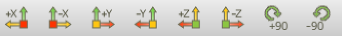
These icons each orient your view along a different Cartesian coordinate axis. The two on the right rotate the camera in fixed ways that changes which direction is up.
In many scenarios, it may be interesting to visually inspect the structure of the mesh on which is defined our data. In the Properties panel, adjust the right option to visualize the mesh as represented as a wireframe drawn on top of the surface cells.
The color coding of the cells turns out to be based on a measure of distance from the center of one of the five cylinders use for bolting the brake to a car. You can use the Threshold filter to extract this cylinder through a careful setting of the maximum value.
Most disc brakes have ventilation slots that are used to transfer heat away during braking, this one is no different. Nevertheless, they are quite hard to see and the Threshold filter does a poor job of extracting them – the problem is that the scalar value defined on vertices does not correlate to their geometry. Instead, we need to address this manually.
ParaView has a filter that can be used to clip arbitrary geometry.
Remove the Threshold filter and instead add a Clip filter. Set the
clipping pane to align with the Y normal and configure it to slice
through the ventilation slots (these look like tiny pillars). Click
apply. Save this state file as A02P03.pvsm. In
A02report.txt answer:
-
Using a wireframe, or Surface w/ Edges allows one to quickly see what type of cell is used in this mesh. What type is it?
-
What is the dimension of this manifold?
-
What were the minimum and maximum values that best captured the single cylinder associated with the bolt’s cylinder?
-
How many ventilation slots are there?
Part 4: Visualizing Unstructured Meshes
Next load, load 3d.vtu. .vtu files encode Unstructured mesh data. Seemingly, this object will look similar to the polygonal mesh we previously saw, but it turns out that this object has a different dimension.
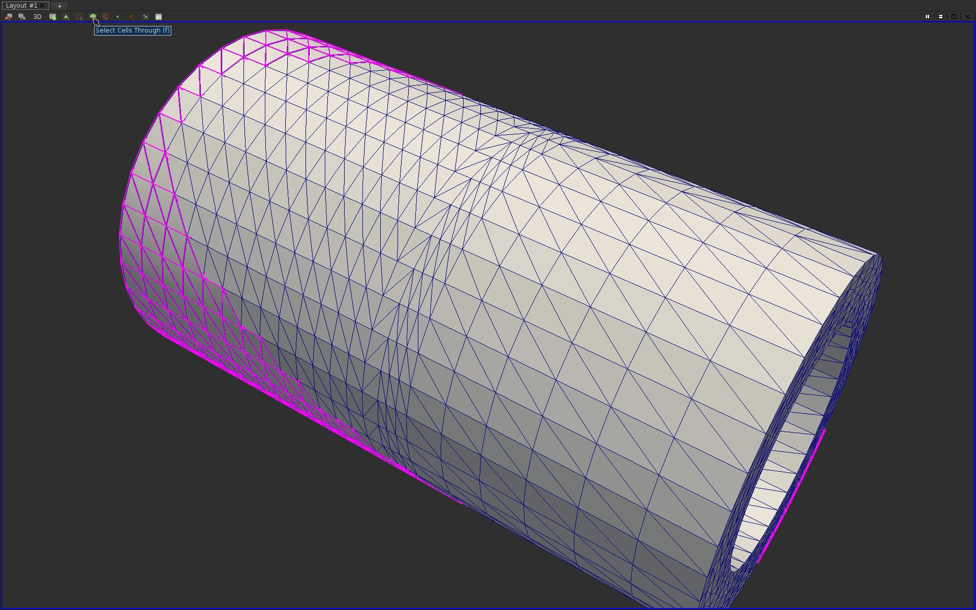
Enabling a Surface with Edges view only enables to display the mesh elements on the boundary of the volume. It is often useful to also inspect the interior of the volume. To achieve this, ParaView provides selection features, which enable users to interactively select regions of interest in the geometry. This selection tool can be extremely useful in variety of other visualization tasks. To use the selection tool, click on the Select Cells Through button at the top of the visualization panel. This tool can also be accessed by hitting the key “f”.
After selecting some parts of the geometry, you should see your selection highlighted in magenta like the following:
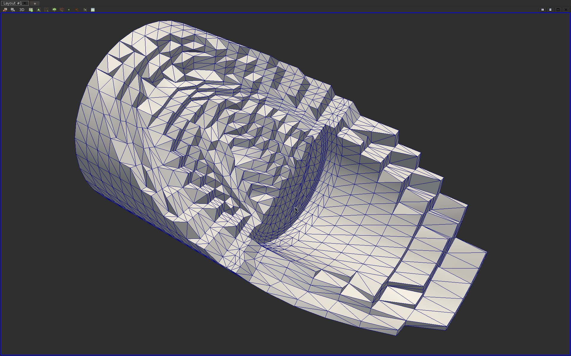
Find and apply the appropriate filter to create a pipeline object that extracts only the selected cells. If you answered correctly this question, here is what you should be visualizing:
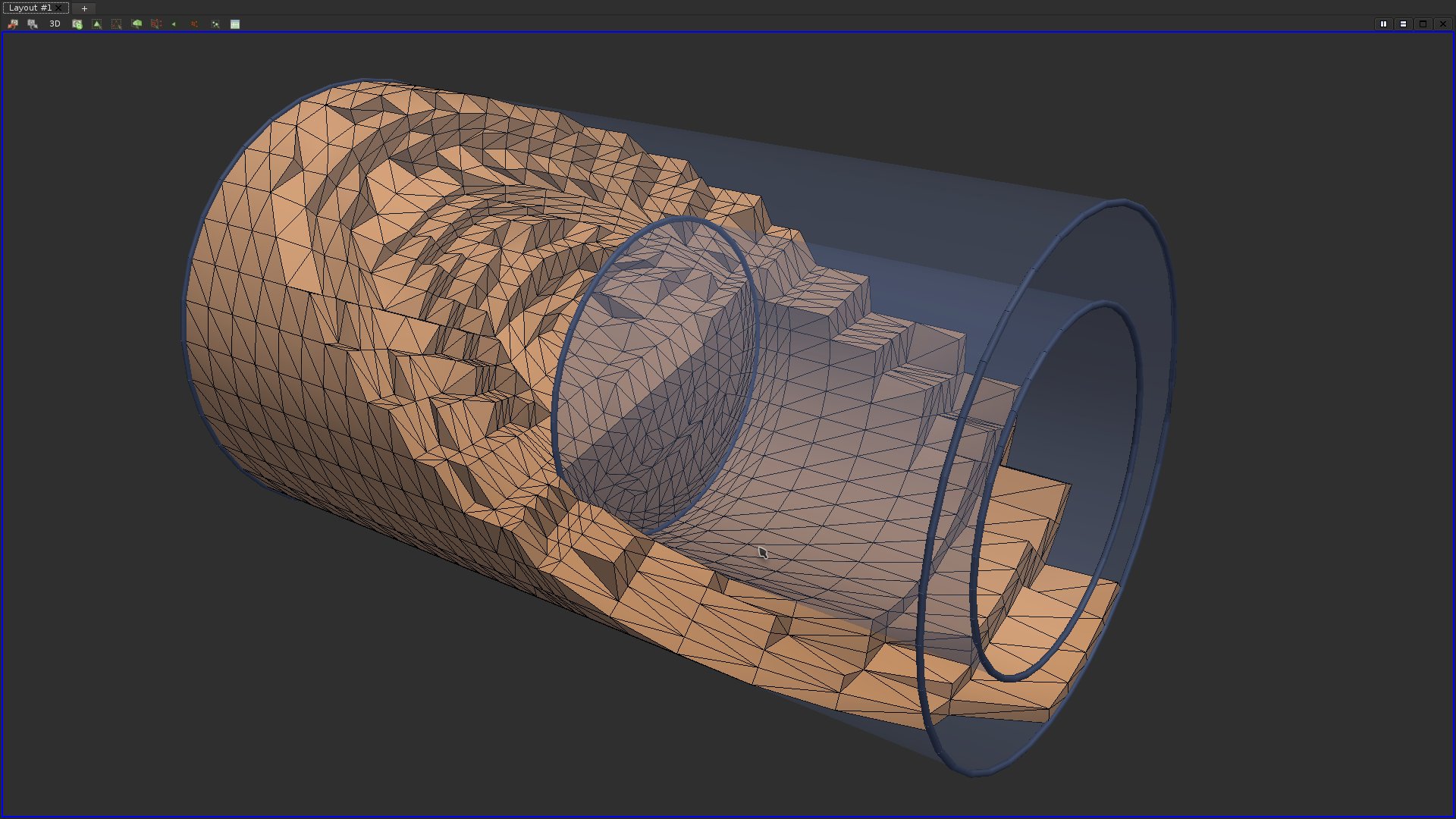
Finally, let’s try to make this view more informative. The Extract Surface filter can be used to extract the boundary surface as a separate polygonal mesh. By adjusting the opacity in the Properties tab, one can make this boundary surface transparent. Next, one can extract feature lines where there are corners (called feature edges) that can be drawn with fattened Tubes using an additional filter. Each of these components can be drawn together by manipulating which are visible in the pipeline browser, and tweaking which Solid Color is used to draw them. Try it out. If you answered correctly this question, here is what you should be visualizing:
Save your best attempt at viewing this as a state file, A02P04.pvsm.
In A02report.txt answer:
-
What dimension is this manifold? What type of cells are used? You may find the SpreadSheet view helpful in answering this question.
-
Is this shape hollow or filled?
Part 5: Visualizing 3D Images
Finally, we’ll try out visualizing a three-dimensional image in
ParaView. Load 3d.vti. You should see only an outline of the
bounding box at this point.
3D images are commonly visualized using axis-aligned slices. ParaView has this capability built in with the Slice filter. Try it out now. Create a slice that is aligned with the X normal of the image. You should see something like this:
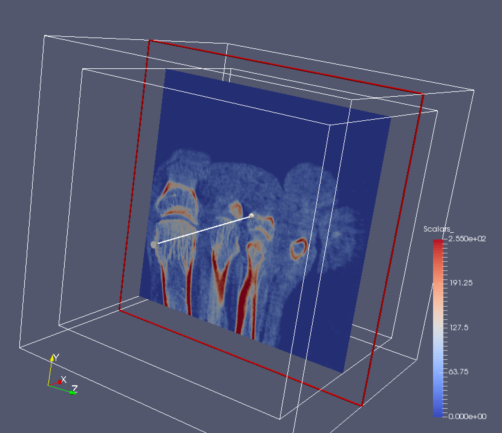
Rotate the dataset and look at the slice from both sides. Note that where you click is important – if you click inside the red square you can actually adjust the depth of the slice. You can also adjust this manually in the Properties panel. You can also rotate the slice if you click on the arrow widget.
Slicing along a single axis is limited in that it only shows you a certain view of the data. Sometimes, it’s helpful to create slices along multiple axes at the same time to get a 3D feel of the data. Create two additional slice filters, one aligned on the Y normal and Z normal of dataset and view all three simultaneously. Rotate the volume around and investigate it.
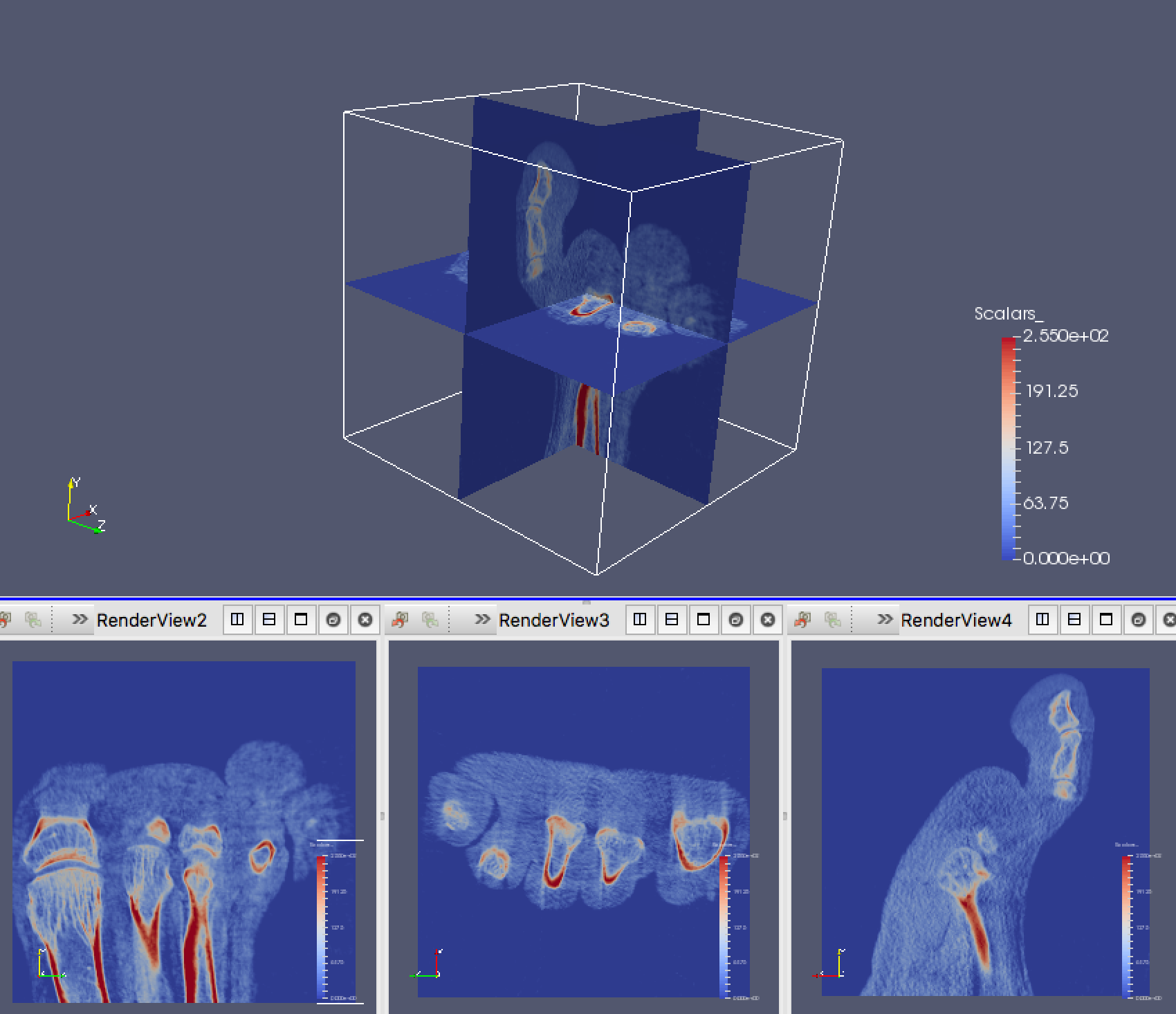
Finally, we’ll create a linked view in ParaView. To do so, we’ll view the same element of the Pipeline Browser in multiple renders. First, split the view vertically so that you have a top and bottom view. Next, in the bottom view, split it horizontally twice to create 3 small views.
One at a time, click on each of the smaller views and make only one of the slices visible. You’ll see that it will default to a 3D render view for these slices. Change this to a 2D view and use the camera controls so that you’ll see the slice head on. You’ve now created a multiple linked view. If you adjust the properties of the slice in one panel, the other views should adjust accordingly.
If you’ve done all of this right, you should have a view that looks like this:
Save your best attempt at viewing this as a state file, A02P05.pvsm.
Grading
My expectation is that you will submit one folder in your git repository
named A02. This folder will contain A02report.txt answering the ten
questions I asked as well as the four ParaView state files I
requested above (for parts 2-5).
I expect the following distribution of points:
- 40% Completing
A02report.txt, each question is worth 4% - 60% Submitting correct ParaView state files. Each of them is worth 15% (there are four total that I request).
This percentage will be scaled to the total value of this assignment for your final grade (7%). Please feel free to include any other documentation of note or comments you would like me to read in your report. Do not submit the data files, these are not necessary to include.