Assignment 06
Flow Visualization
Due: Nov. 29, 2023 03:29:59 PM
Graded: Dec. 06, 2023
Percentage of Grade: 9%
Assignment Description: Finalized
- Objectives
- Preliminaries
- Setting up your visualization
- Part 1: Creating vector field glyphs
- Part 2: Creating streamlines
- Part 3: Controlling the seeding positions
- Written Questions (worth 25/90 points)
- Submission
- Grading
- Extra Credit
In this assignment, you will write code to visualize two-dimensional vector fields through the use of color, glyphs, and geometric features (streamlines). Each of these visual encodings will be used to show different properties of the vector field in different combinations.
Please click here to create your repository
Objectives
This assignment is designed to teach you the basics of vector field visualization through encoding per-position properties with a variety of techniques. Specific objectives include:
- Using color and glyphs to encode both magnitude and orientation.
- Using streamlines to capture integrated properties of streamlines.
- Experimenting with both random and uniform seeding patterns to adjust the position of both glyphs and streamlines
- Further practice in using SVG shapes, d3 scales, and integrating d3.js and vtk.js
Preliminaries
We will visualize two-dimensional vector field datasets included in the datasets folder as .vti files. As in A05, you may want to experiment with visualizing these in ParaView. By default, when loading these files ParaView will display them by color mapping the magnitude of the vector field at each point. You could also try out the “Glyph” and “Stream Tracer” filters from the Filter menu.
We have provided a class, in the file flowvis.js that is designed to load and provide access to the vector field. You’ll see that index.html and a06.js are set up similarly to A05 with a file open dialog. Upon loading one of the .vti files, an instance of this class vfImageInterpolator is returned. This class provides one key function you will use, interpolate(x,y) that returns a list with two values, [vx,vy], with the vector value \((v_x,v_y)\) at the position \((x,y)\).
Positions are passed to interpolate() in world coordinates, based on the size of the vector field’s domain in geometry coordinates. They need not lie on sample points – my interpolate method will return the bilinear interpolation of the four nearest points. If the position \((x,y)\) is outside of the bounds of the vector field, I will return the vector \((0,0)\)
Besides this function, the class vfImageInterpolator also stores some important properties you will use in setting up your visualization. Particularly, the property bounds returns the world coordinates size of the domain. Particularly, bounds[0] is the minimum \(x\)-coordinate, bounds[1] is the maximum \(x\)-coordinate, bounds[2] is the minimum \(y\)-coordinate, and bounds[3] is the maximum \(y\)-coordinate. The property range returns the minimum and maximum magnitude of the vector field as range[0] and range[1]. There are some additional variables, such as dims and extent that refer to the size of the input grid, but you will likely not use this variables, as well as internal variables that store the raw vector data.
Setting up your visualization
Your visualization must allow the user to view the vector field using both glyphs and streamlines. Both glyphs and streamlines must be allowed to be placed at uniformly distributed positions over the vector field domain as well as random positions.
In addition, your visualization should make it clear what the geometric size of the vector field domain is. To do this, I’ve suggested that you use the aspect ratio of input domain to resize the SVG element. Particularly, I recommend that you keep the width of the plot fixed (in my implementation I set it to be 800) and then resize the height of the plot to be relative to the aspect ratio.
Besides making sure the geometry of the visualization respects the domain size, I also recommend creating scales for both the \(x\)- and \(y\)-coordinate space. You will need these scales to map from positions in the vector field domain to positions on the screen. This way, when you access the vector field information (e.g. in a call to interpolate()) you can use the coordinate system of the vector field itself, but when you draw the vector field, you can map these positions using your scales.
Besides this, you can also use these scales to construct axes that show the geometric bounds of the vector field domain.
Part 1: Creating vector field glyphs
Your first visualization mechanism will be to draw glyphs that show the vector variables at a collection of points within the domain. To do this, you will need to create a list of positions where you want to draw the glyphs. Next, you can then use a data join on these positions where you call the function interpolate() to access the vector value at that position.
Your glyphs can be anything you choose, but they must encode both the direction of the vector and its magnitude. You can encode these two properties redundantly if you’d like, for example using color, size, and/or geometry.
I found it helpful to create additional scales for color and magnitude, based on the property range stored in the vfImageInterpolator class. Particularly, the magnitude scale was helpful since the vectors in the various datasets all have very different magnitudes. Recall that the magnitude of a vector can be computed as \(\sqrt{v_x^2 + v_y^2}\). Using the magnitude scale, I could map from vector lengths to pixel lengths, and thus control the visual size of the glyphs. A successful default implementation, on the Bickley jet dataset, might look something like this:
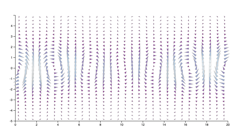
A few hints on drawing glyphs in this way.
- It may help to consider drawing glyphs in multiple pieces. For example, if you choose to draw an arrow you could draw two pieces for each arrow, using a separate SVG path for the stem and head of the arrow. This isn’t necessary, but I found it easier to think about.
- It’s easier to draw the glyph pointing in one fixed direction, and then rotate the entire arrow using the appropriate SVG commands. You will also likely want to use Math.atan2 to compute the angle of this rotation.
- SVG transform attributes can have more than one instruction. See the example “Rotating and translating and SVG element” in the MDN documentation.
Part 2: Creating streamlines
After experimenting with glyphs, your next task is to create an interface for the user to draw streamlines on the flow field. To do this, you will implement the Runge-Kutta 4 method as described in class (see L22). Perhaps the most straightforward way to do this is to compute a list of pairs of \((x,y)\) positions on the streamline, e.g. list = [[x0,y0],[x1,y1],...] and then pass this list to a call of d3.line()(list) to produce the d attribute for an SVG path element.
To do this, you will have to implement a method for interpolation on the streamline. In my implementation, I did this by writing a function with the signature rk4Integrate(start) that took as input a start position start and produced such a list. In addition to needing access to the vector field’s interpolate() method, this function also requires two variables: dt, or the amount of time each step takes and numSteps, or the number of steps you will integrate.
Setting defaults for these numbers can be tricky, especially for vector fields defined on various sized domains and with varying ranges of magnitudes. I found it helpful to think of dt as something like “how much time would it take to walk across the domain at the average speed of the vector field?”. Thus, using bounds and range, I could estimate a reasonable default dt, and then scale it based on how many steps. Feel free to experiment here, or better, give the user an interface to adjust the numbers.
If you implement it this way, rk4Integrate() will produce a set of positions in the coordinate space of the vector field’s domain. Using the scales for the \(x\)- and \(y\)-coordinates, you can then convert these positions to the screen coordinates to finally draw the streamlines. A successful default implementation, again on the Bickley jet dataset, might look something like this:
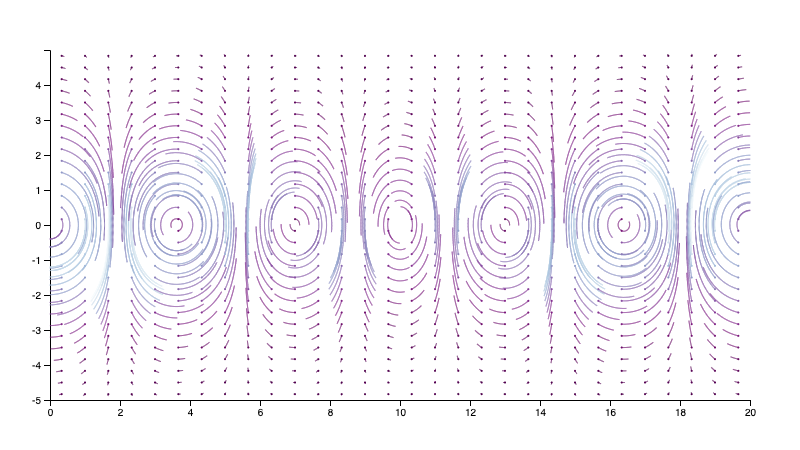
Note that, since interpolate() returns \((0,0)\) for a position outside of the domain, you can use this to optimize your integration method. Particularly, if you ever encounter a vector value of \((0,0)\) you know that there is no reason to continue integrating, as a zero magnitude vector means that the field has stopped at this position. Thus, you can stop the loop early rather than integrating for the full number of numSteps.
Part 3: Controlling the seeding positions
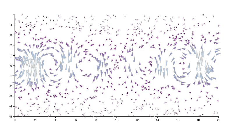
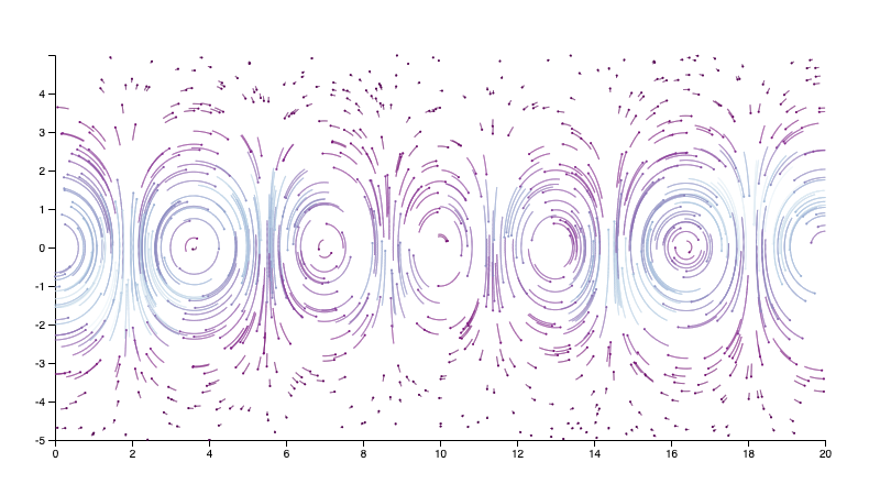
Finally, you must implement two different mechanisms for deciding the positions of glyphs and streamline seeds. In the previous images, I used a uniform distribution of positions over a grid.
Your visualization must allow the user to also specify seed positions at random locations. When complete, this would create visualizations that look something like the following:
Written Questions (worth 25/90 points)
-
Given a full description of the visual encoding you used for your glyph design in this assignment. Which properties of the vector field did you map to which visual channels, and why?
-
In two dimensions, what possible topological changes occur for isocontours at critical points that are saddles?
-
What is a limitation of using a texture-based approach such as LIC to visualize flow fields as compared with geometric techniques? What is a strength?
Submission
You should use git to submit all source code files. The expectation is that your code will be graded by cloning your repo and then executing it within a modern browser (Chrome, Firefox, etc.)
Please provide a README.md file that provides a text description of how to run your program and any parameters that you used. Also document any idiosyncrasies, behaviors, or bugs of note that you want us to be aware of.
To summarize, my expectation is that your repo will contain:
- A
README.mdfile - A
index.htmlfile - An
a06.jsfile - All other Javascript files necessary to run the code (including
flowvis.js,vtk.js, andd3.jsplus any others you require) - Any
.cssfiles containing style information
Grading
Deductions
| Reason | Value |
| Bugs or syntax errors | Up to -10 each bug at grader's discretion to fix |
Point Breakdown of Features
| Requirement | Value | ||||||||||
| External documentation (README.md) following the template provided in the base repository | 5 | ||||||||||
| Consistent modular coding style, indentation, etc. | 5 | ||||||||||
| Header documentation and internal documentation (Block for functions and Inline descriptive comments). Wherever applicable / for all files | 5 | ||||||||||
Expected output / behavior based on the assignment specification, including
| 50 | ||||||||||
Written Questions
| 25 | ||||||||||
| Total | 90 | ||||||||||
Cumulative Relationship to Final Grade
Worth 9% of your final grade
Extra Credit
Implementing features above and beyond the specification may result in additional extra credit, please document these in your README.md.
Bonus points will be awarded for creative use of glyphs and/or streamlines that encode information from the vector field, as well as creative combinations of positioning them. The examples in the above images are just meant as guidelines – there is no need to reproduce them exactly.
Particularly, there are many ways to augment this visualization using more interactive visualization. Think creatively about trying out different ideas with glyphs as well as letting the user specify properties in the visualization (including glyph location, number of steps, and delta t). Another option might be to specify an interactive probe that let’s the user click to draw a glyph and/or streamline at a fixed position.