Assignment 10
Marching Squares
Due: Apr. 15, 2020 03:29:59 PM
Graded: Apr. 22, 2020
Percentage of Grade: 6%
Assignment Description: Finalized
- Objectives
- Description
- Part 1: Implementing Contour Outlines
- Part 2: Implementing Filled Contours
- Submission
- Grading
- Extra Credit
In this assignment, you will write code to visualize two-dimensional scalar fields through the use of contours. Contours will be constructed using the Marching Squares algorithm discussed in class. Your main task will be to implement this algorithm.
Please click here to create your repository
Objectives
This assignment is designed to teach you the basics of scalar field visualization through combinations of geometric features (isocontours) and color mapping. Specific objectives include:
- Implementing the marching squares algorithm for extracting isocontours in a piecewise manner.
- Utilizing a case-table structure to maintain repeated computational structure and develop the algorithm in a compact way
- Further practice in using SVG paths and d3’s features for constructing them
- Experimenting with visual encoding of scalar fields utilizing both isocontour outlines and filled isocontours.
Description
We will again attempt to visualize a weather simulation of Hurricane Isabel that we used in A06. This dataset is stored in the file data.js, but instead of using the array data, we will mostly focus on two arrays, temperatureCells and pressureCells. Each array contains objects that look like:
{
    NW: value-at-nw-corner,
    NE: value-at-ne-corner,
    SW: value-at-sw-corner,
    SE: value-at-se-corner,
    Row: i,
    Col: j
}
So, unlike A06, the main selections we are doing will be cell-focused rather than vertex-focused. Thus, each element you draw will be based on the collection of four values stored in the four corners (northwest (NW), northeast (NE), southwest (SW), and southeast (SE) of the cell, rather than just drawing each data value as one square. Thus, instead of having a grid of \(50\times50\) squares, this assignment will process the data as a grid of \(49\times49\) cells.
Before writing the full marching squares code in Parts 1 and 2, we recommend that you try to understand at a high level what the template code is doing. A good way to start is to write code that adds a fixed, small shape inside of each square regardless of what case the cell corresponds to.
Part 1: Implementing Contour Outlines
First, you will implement the computation of outline contours using marching squares. To do this, you will complete the skeleton code function generateOutlineContour() in a10.js. This function should return an SVG path specifier (the d attribute) for the contour located at a given cell d. When successfully implemented, you should see images that look like:
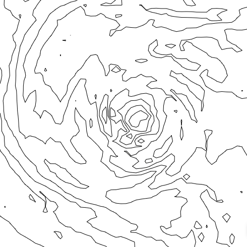 |
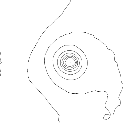 |
| Temperature Contours | Pressure Contours |
Note that, like in A06 we have spaced out each cell to be exactly \(10\times10\) pixels. So, within generateOutlineContour(), you should return a path specified using units between \([0,10]\) for both the \(x\)- and \(y\)-coordinates. We have provided transformations so that the position \((0,0)\) in the local coordinate space for each cell corresponds to the SW value, and the position \((10,10)\) corresponds to the NE value.
Thus, the way the skeleton code is set up, the path for each separate square can be specified in a “local” coordinate system (use your web browser’s debugger to inspect the DOM after executing the skeleton code and pay attention to the “transform” nodes in each of the g elements). In other words, you should not have to write code to decide on what position along the SVG each square should be drawn.
You may choose to generate the SVG path specifier however you please. The string that you return must be in SVG path syntax, so you can write functions for this on your own. Alternatively, you could also use d3.line() to compute this string, similar to in past assignments. Note that for certain cases, you may need to return multiple, disconnected lines, so if you use d3 you may need to use the .defined() function to create breaks in the line.
Part 2: Implementing Filled Contours
Second, you will implement the computation of filled contours, again used a marching squares to compute the boundary of contours. To do this, you will complete the skeleton code function generateFilledContour() as well as the function includesFilledContour() in a10.js. When successfully implemented, you should see images that look like:
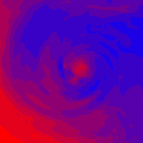 |
 |
| Temperature Filled Contours | Pressure Filled Contours |
You will have to take care to notice the order in which filled contours are draw. In this case, we will draw multiple, overlapping contours and rely on the order in which they are drawn to see them visually. Particularly, the function createFilledPlot() draws the contours will highest value first and then layers the lower values on top of them.
Thus, unlike with Part 1, you need draw something for a different set of cells, that you will select with includesFilledContour(). And, the case table that you produce in generateFilledContour() must provide the full outline for the polygon that spans the cell, rather than just the polyline that lives on its border.
All visual characteristics, such as the color map used to set the fill color, have been provided for you and you should not need to modify these.
Submission
You should use git to submit all source code files. The expectation is that your code will be graded by cloning your repo and then executing it within a modern browser (Chrome, Firefox, etc.)
Please provide a README.md file that provides a text description of how to run your program and any parameters that you used. Also document any idiosyncrasies, behaviors, or bugs of note that you want us to be aware of.
To summarize, my expectation is that your repo will contain:
- A
README.mdfile - A
index.htmlfile - An
a10.jsfile - All other Javascript files necessary to run the code (including
data.jsandd3.v5.jsplus any others you require) - Any
.cssfiles containing style information
Grading
Deductions
| Reason | Value |
| Bugs or syntax errors | -10 each bug at grader's discretion to fix |
Point Breakdown of Features
| Requirement | Value | ||||||||||
| Consistent modular coding style | 5 | ||||||||||
| External documentation (README.md) following the template provided in the base repository | 5 | ||||||||||
| Header documentation, Internal documentation (Block for functions and Inline descriptive comments). Wherever applicable / for all files | 10 | ||||||||||
Expected output / behavior for your chart based on the assignment specification, including
| 80 | ||||||||||
| Total | 100/100 | ||||||||||
Cumulative Relationship to Final Grade
Worth 6% of your final grade
Extra Credit
Implementing features above and beyond the specification may result in additional extra credit, please document these in your README.md. Particularly, you may want to consider additional user interface features that allow you to select a different number of contours or otherwise inspect the data more closely.